这真的是一个题目
近些天沉迷wow,实在是太好玩了。
最近还在准备六级,这次必定拿下六级。
认识了一个成都的小姐姐真开心啊!
还有这个1km跑步始终是个梗,不知道是身体变差了还是老了。加油加油~
那就下次再见吧。
K最近邻(k-Nearest Neighbor,KNN)分类算法,是一个理论上比较成熟的方法,也是最简单的机器学习算法之一。该方法的思路是:如果一个样本在特征空间中的k个最相似(即特征空间中最邻近)的样本中的大多数属于某一个类别,则该样本也属于这个类别。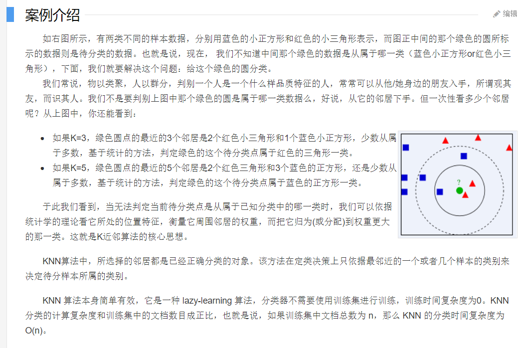
import numpy as np
import matplotlib.pyplot as plt

# 初始化模拟数据
# X_train 为样本点
X_train = np.array([[2, 1],[3, 2],[4, 2],[1, 3],[1.5, 4],[1.7, 3],[2.6, 5],[3.4, 3],
                    [3, 6],[1, 7],[4, 5],[1.2, 6],[1.8, 7],[2.2, 8],[3.7, 7],[4.8, 5]])
# y_train 为样本点标记
y_train = np.array([0,0,0,0,0,0,0,0,1,1,1,1,1,1,1,1])
# X_test 为测试样本
X_test = np.array([3.2, 5.4])
# k 为邻居数
k = 3

# 这里的距离公式采用欧式距离
square_ = (X_train - X_test) ** 2
square_sum = square_.sum(axis=1) ** 0.5
# 根据距离大小排序并找到 测试样本 与 所有样本k个最近的样本的序列
square_sum_sort = square_sum.argsort()
small_k = square_sum_sort[:k]
# K近邻用于分类则统计K个邻居分别属于哪类的个数,用于回归则计算K个邻居的y的平均值作为预测结果
# 统计距离最近的k个样本 分别属于哪一类的个数 别返回个数最多一类的序列 作为预测结果
y_test_sum = np.bincount(np.array([y_train[i] for i in small_k])).argsort()
# 打印预测结果
print('predict: class {}'.format(y_test_sum[-1]))

# 将数据可视化 更生动形象
# 将 class0 一类的样本点 放到 X_train_0中
X_train_0 = np.array([X_train[i, :] for i in range(len(y_train)) if y_train[i] == 0])
# 将 class1 一类的样本点 放到 X_train_1中
X_train_1 = np.array([X_train[i, :] for i in range(len(y_train)) if y_train[i] == 1])

# 绘制所有样本点 并采用不同的颜色 分别标记 class0 以及 class1
plt.scatter(X_train_0[:,0], X_train_0[:,1], c='g', marker='o', label='train_class0')
plt.scatter(X_train_1[:,0], X_train_1[:,1], c='m', marker='o', label='train_class1')
if y_test_sum[-1] == 0:
    test_class = 'g'
elif y_test_sum[-1] == 1:
    test_class = 'm'
plt.scatter(X_test[0], X_test[1], c=test_class, marker='*', s=100, label='test_class')
# 连接 测试样本 与k个近邻
for i in small_k:
    plt.plot([X_test[0], X_train[i, :][0]], [X_test[1], X_train[i, :][1]], c='c')
plt.legend(loc='best')
plt.show()English version
Chinese version
tf.train API
一个简单的线性回归
import numpy as np
import tensorflow as tf
#Model parameters
W = tf.Variable([.3], dtype=tf.float32)
b = tf.Variable([-.3], dtype=tf.float32)
#Model input and output
x = tf.placeholder(tf.float32)
linear_model = W * x + b
y = tf.placeholder(tf.float32)
#loss
loss = tf.reduce_sum(tf.square(linear_model - y)) # sum of the squares

#optimizer,定义一个优化器,使用梯度下降优化方法
optimizer = tf.train.GradientDescentOptimizer(0.01)
#优化器最小化loss
train = optimizer.minimize(loss)

#training data
x_train = [1,2,3,4]
y_train = [0,-1,-2,-3]

#training loop
init = tf.global_variables_initializer()
sess = tf.Session()
sess.run(init) # reset values to wrong

#迭代一千次后,参数已经训练好
for i in range(1000):
sess.run(train, {x:x_train, y:y_train})

#送入训练好的参数,求出loss
#evaluate training accuracy
curr_W, curr_b, curr_loss = sess.run([W, b, loss], {x:x_train, y:y_train})
print("W: %s b: %s loss: %s"%(curr_W, curr_b, curr_loss))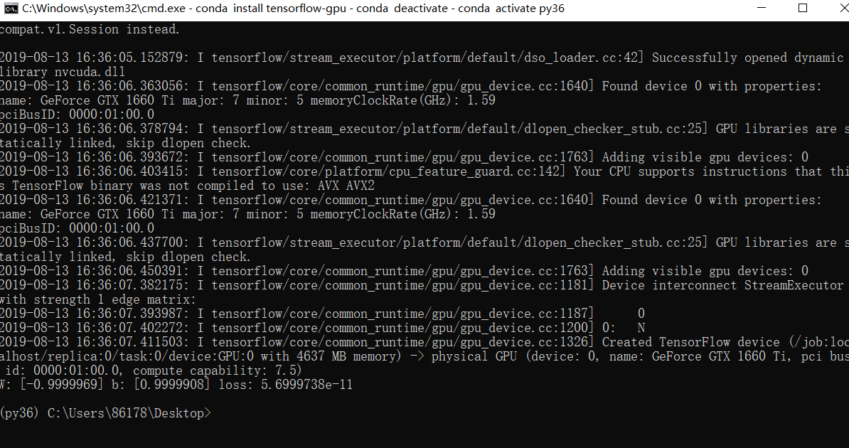
Welcome to Hexo! This is your very first post. Check documentation for more info. If you get any problems when using Hexo, you can find the answer in troubleshooting or you can ask me on GitHub.
1 | $ hexo new "My New Post" |
More info: Writing
1 | $ hexo server |
More info: Server
1 | $ hexo generate |
More info: Generating
1 | $ hexo deploy |
More info: Deployment